Mode Solver
API Documentation
Vector Finite-Difference Mode Solver |
|
Mode Solver Results class. |
Dielectric Waveguide Mode Analysis
This example uses the gdstk module to create a GDSII file, sets some constant materials for use as substrate, background and waveguide filling materials. After that, it sets the
device geometry using the .gds file with 1 micron padding all around.
Finally the solver is instanced and the settings that follow are used to setup the proper cross section cut for mode analysis.
The cut is set to the YZ plane as the propagation happens along X. Then we set cut location to 0 (along the x-axis) that
according to the .gds file corresponds to the beginning of the dielectric waveguide. The wavelength is set from 1.5-1.6 microns, the initial guess to 3.4
and the number of modes (nmodes) to 4. the tolerance is set to 1e-8 (0.0 would mean machine precision).
The mode solver solves for the H-fields first. Setting the boundaries to PMC, enforces tangential H-fields to the boundaries of the cross section to be zero. Other boundary options can be found in SetSimSettings <pyModeSolver.pyModeSolver.VFDModeSolver.SetSimSettings>.
The results are set to be saved in the ModeResults folder with the name my_results. If multiple simulations are run, and the res_filename
already exists, the solver will append date and time to make it unique.
The Run command is called to start the simulation, that returns a ModeSolverResults <pyModeSolver.ModeSolverResults.ModeSolverResults> object.
You can check it for detailed members and methods. Overall it provides an easy and pythonic way of navigating through the results.
For example:
<results>.PlotMode()will provide the field profile of a mode at a given frequency.<results>.PlotPermittivity()will allow you to visualize the cross section permittivity profile.<results>.PlotIndex('neff')will plot the modes effective refractive index for one or multiple modes.<results>.PlotIndex('ng')will plot the modes effective group index for one or multiple modes.<results>.Polarity()will print the polarity of the modes at the specified wavelength.
from pyModeSolver.pyModeSolver import VFDModeSolver
from pyOptiShared.LayerInfo import LayerStack
from pyOptiShared.DeviceGeometry import DeviceGeometry
from pyOptiShared.Material import ConstMaterial
import gdstk
import numpy as np
import matplotlib.pyplot as plt
##########################################
### WG GDS File ###
##########################################
filename = "wg.gds"
length = 10
width1 = 0.5
width2 = 2
lib = gdstk.Library()
strt_wg = lib.new_cell("Straight_WG")
vertices1 = [(0, -width1/2), (length, -width1/2), (length, width1/2), (0, width1/2)]
vertices2 = [(0, -width2/2), (length, -width2/2), (length, width2/2), (0, width2/2)]
strt_wg.add(gdstk.Polygon(vertices1, layer=1))
strt_wg.add(gdstk.Polygon(vertices2, layer=2))
lib.write_gds(filename)
##########################################
### Material Settings ###
##########################################
substrate_mat = ConstMaterial("SiO2", epsReal=1.444**2, epsImag=0.0)
core_mat = ConstMaterial("Si", epsReal=3.48**2, epsImag=0.0)
##########################################
### Layer Stack Settings ###
##########################################
layer_stack = LayerStack()
layer_stack.AddLayer(number=1,material=core_mat, thickness=0.22, zmin=0, sideWallAng=0, cladding="Air_default")
layer_stack.AddLayer(number=2,material=core_mat, thickness=0.09, zmin=0.0, sideWallAng=0, cladding="Air_default")
layer_stack.SetBGandSub(background="Air_default", substrate=substrate_mat)
##########################################
### Device Geometry/Port Settings ###
##########################################
device_geometry = DeviceGeometry()
device_geometry.SetFromGDS(layer_stack=layer_stack,
gds_file=filename,
buffers={'x':1,'y':1,'z':1})
##########################################
### ModeSolver Settings ###
##########################################
mode_solver = VFDModeSolver()
mode_solver.SetBoundaries(min_x = "pmc", max_x = "pmc",
min_y = "pmc", max_y = "pmc")
lams=np.linspace(start=1.5,stop=1.6,num=5)
mode_solver.SetSimSettings(device_geometry = device_geometry,
mesh={"dx": 0.02,"dy": 0.02, "dz": 0.02},
wavelength=lams,
nguess = 2.1,
nmodes = 10,
cut_plane = "YZ",
cut_location = 0.0,
tol = 1e-8,
results_path = "./ModeResults",
device_name = "my_results")
##########################################
### Run and Results Visualization ###
##########################################
results = mode_solver.Run()
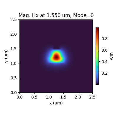
results.PlotMode(field='Hy') # Fundamental Mode Profile
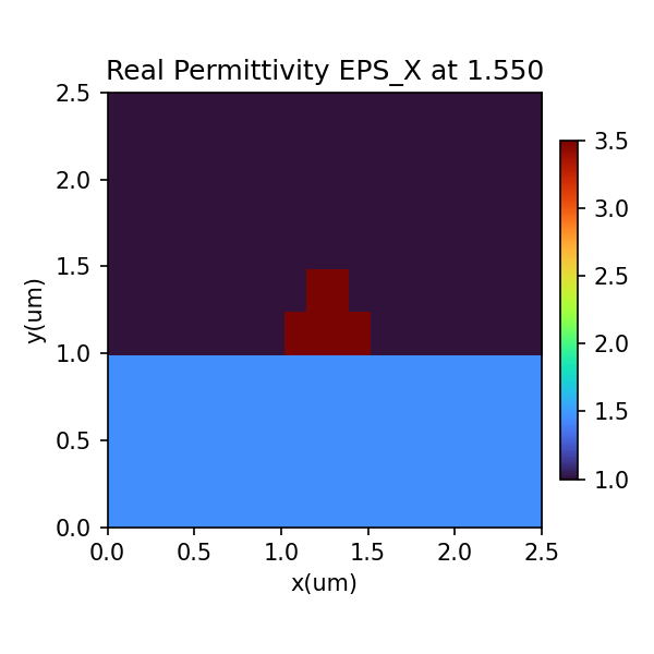
results.PlotPermittivity() # Material Profile
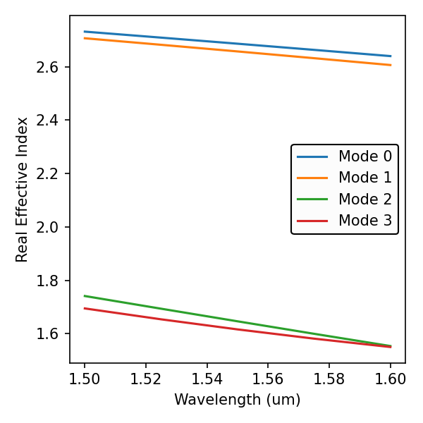
results.PlotIndex('neff',modes=[0,1,2,3]) # Effective Refractive Index
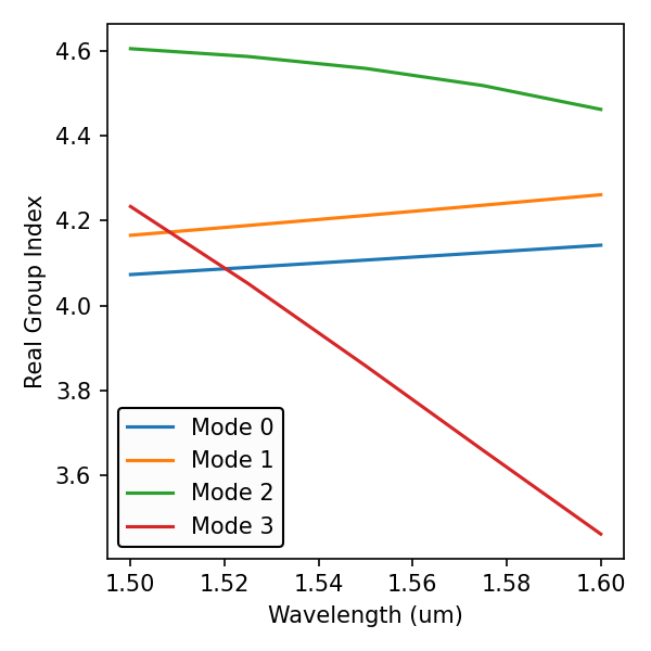
results.PlotIndex('ng',modes=[0,1,2,3]) # Effective Group Index
results.Polarity(wavelength=1.5) # polarity of the modes
plt.show()
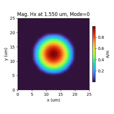
Fiber - XY Cut Mode Analysis
This example uses the gdstk module to create a GDSII file of a fiber and then compute its mode profile.
import gdstk
import os
from pyModeSolver.pyModeSolver import VFDModeSolver
from pyOptiShared.LayerInfo import LayerStack
from pyOptiShared.DeviceGeometry import DeviceGeometry
from pyOptiShared.Material import ConstMaterial,ExperimentalMaterial
import numpy as np
import matplotlib.pyplot as plt
##########################################
### Create Fiber GDS File ###
##########################################
filename = "fiber.gds"
lib = gdstk.Library()
cell = lib.new_cell("fiber")
circle = gdstk.ellipse((0, 0), 7.5,layer=1)
cell.add(circle)
lib.write_gds(filename)
##########################################
### Material Settings ###
##########################################
air_mat = ConstMaterial("air", epsReal=1, epsImag=0.0)
sio2_exp = ExperimentalMaterial("my_material")
sio2_exp.SetFromRefDotInfo(shelf="main", book="SiO2", page="Malitson", wavelength_unit=1e-6)
##########################################
### Layer Stack Settings ###
##########################################
layer_stack = LayerStack()
layer_stack.AddLayer(number=1,material=sio2_exp, thickness=0.0, zmin=0, sideWallAng=0, cladding=air_mat)
layer_stack.SetBGandSub(background=air_mat, substrate=air_mat)
##########################################
### Device Geometry/Port Settings ###
##########################################
device_geometry = DeviceGeometry()
device_geometry.SetFromGDS(layer_stack=layer_stack,
gds_file=filename,
buffers={'x':5,'y':5,'z':5})
##########################################
### ModeSolver Settings ###
##########################################
lams=np.linspace(start=1.5,stop=1.6,num=5)
mode_solver = VFDModeSolver()
mode_solver.SetBoundaries(min_x = "pmc", max_x = "pmc",
min_y = "pmc", max_y = "pmc")
mode_solver.SetSimSettings(device_geometry = device_geometry,
mesh={"dx": 0.5,"dy": 0.5, "dz": 0.5},
wavelength=lams,
nguess = 3.4,
nmodes = 1,
cut_plane = "XY",
cut_location = 0.0,
tol = 1e-8,
results_path = "./ModeResults",
device_name = "my_results")
##########################################
### Run and Post Processing ###
##########################################
results = mode_solver.Run()
## Built in plotting functions
results.PlotMode() # Fundamental Mode Profile
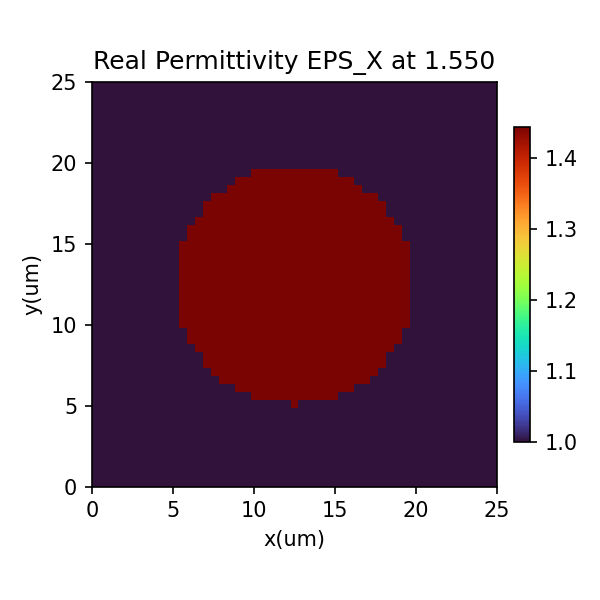
results.PlotPermittivity() # Material Profile
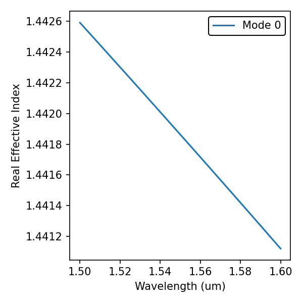
results.PlotIndex('neff',modes=[0]) # Effective Refractive Index
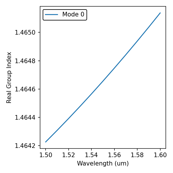
results.PlotIndex('ng',modes=[0]) # Effective Group Index
plt.show()