NXData Data Class

Overview 

In order to store simulation results we provide them in the .hdf5 format. Which a versatile and efficient way to organize and store data and metadata. To improve data visualition, we whent further and provided initial support to the NeXus format, that allows to organize data even further, including metadata and better support to results visualization.

The NXdata dataclass is the object that is used to store our solver restults. In general you can access data based on the NeXus format (signal, auxiliary_signals, axes, etc), and to facilitated its visualization we provide the Plot method to easily provide a data visualization interface for the user.

Examples 

Visualization of FDTD Results 

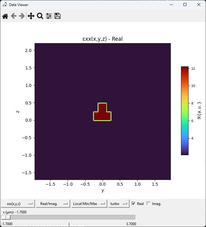
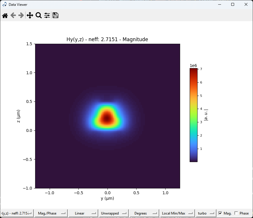
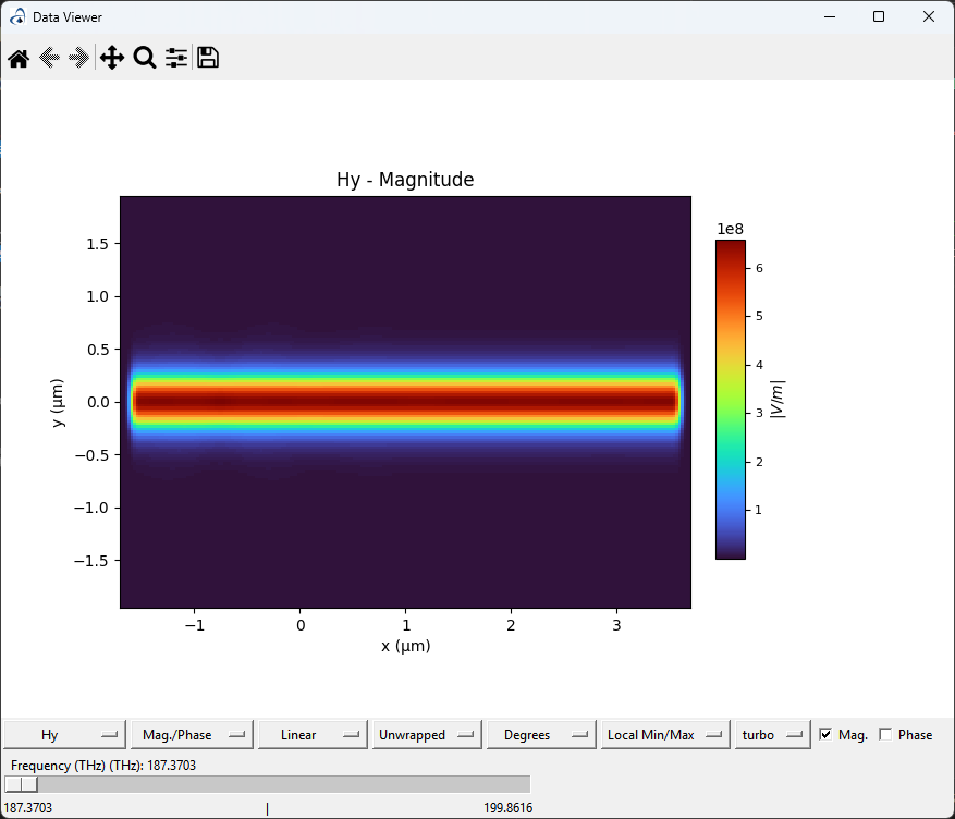
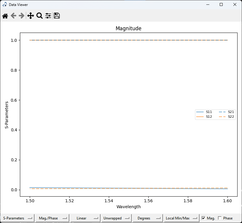
This example relies on the FDTD Solver and the FDTDSimResults. The .hdf5 with the results can be downloaded here: wg_results_fdtd.hdf5. The results shown are the permittivity profile, mode profile on Mode Source o1, DFT field progile of MyFDTMonitor1 and ALL the scattering parameters.

from pyOptiShared.SimResults import FDTDSimResults
import sys

filename=r"wg_results_fdtd.hdf5"
results = FDTDSimResults()
results.loadHDF5(filename)

#Python is not running in ipykernel. Desktop plotting tools can be used with NXDATA
if 'ipykernel' not in sys.modules:
        results.permittivity.Plot()
        results.mode_sources["Mode Source o1"].fields.Plot()
        results.runs[0].dftmonitors["MyDFTMonitor1"].Plot()
        results.sparameters["ALL"].Plot()
else: #Otherwise fall back to using basic matplotlib
        results.PlotPermittivity(cut='x',position=0.5)
        results.PlotDFTMonitor('Mode Monitor o1',run_num=0,field='Hy')
        results.PlotDFTMonitor('MyDFTMonitor1',run_num=0,field='Hy')
        results.PlotSParameters('ALL')

FDTD Permittivity Cross Section

Mode Profile ‘Mode Source o1’

DFT Monitor Field View

Scattering Parameter Results

Visualization of Mode Solver Results 

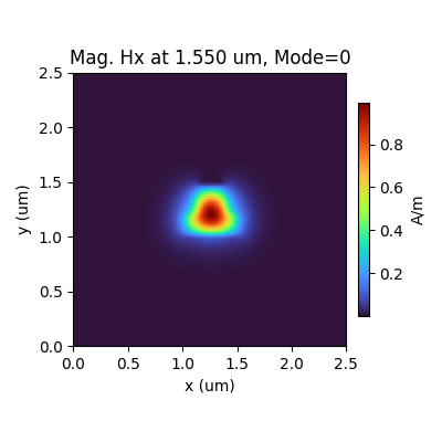
This example relies on the Mode Solver and the ModeSolverResults classes. The .hdf5 with the results can be downloaded here: wg_results_mode.hdf5. The data we are showing is the mode profile of Hy for the fundamental mode (index equals 0) for the same dielectric waveguide example as the one in the previous example.

from pyOptiShared.SimResults import ModeSolverResults
import sys

filename=r"wg_results_mode.hdf5"
results = ModeSolverResults()
results.loadHDF5(filename)

#Python is not running in ipykernel. Desktop plotting tools can be used with NXDATA
if 'ipykernel' not in sys.modules:
        results.fields.Plot()
        results.material_grid.Plot()
        results.neff.Plot()
        results.ng.Plot()
else: #Otherwise fall back to using basic matplotlib
        results.PlotMode() # Fundamental Mode Profile
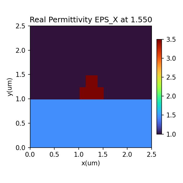
        results.PlotPermittivity()  # Material Profile
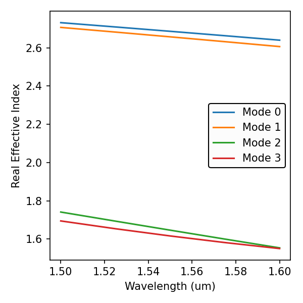
        results.PlotIndex('neff',modes=[0,1,2,3]) # Effective Refractive Index
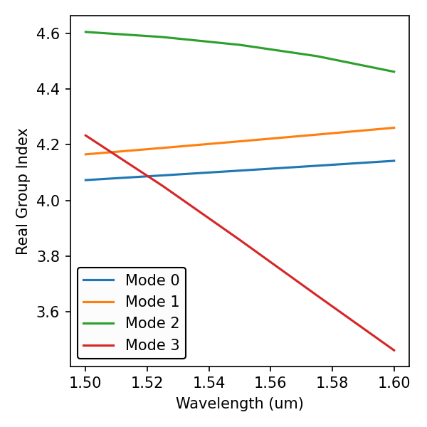
        results.PlotIndex('ng',modes=[0,1,2,3]) # Effective Group Index